MATLAB Introduction

This week we started to learn MATLAB by reading the first chapters of Physical Modeling in MATLAB by Allen Downey and doing some exercises from the book.

The first exercise 2.1 was to translate the equation of the nth number of the fibonacci sequence in MATLAB.

2.3- calculate the number of cars in two locations, Boston and Albany, of a rental car company each week. Each week 5% of the cars in Albany are dropped off in Boston and 3% of the cars in Boston are dropped off in Albany. This script updates the number of cars in Boston and Albany each week. At the beginning of the year, 150 cars are at both locations.

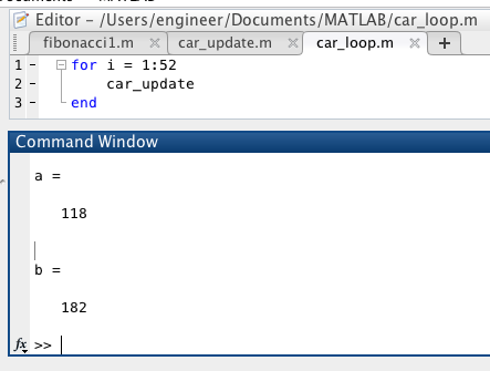
Exercise 3:1- Use the for loop to run car.update 52 times. This would tell us how many cars will be in Boston and Albany at the end of the year. The year starts with 150 cars in Boston and 150 cars in Albany.

Exercise 3:2- We modified the car_loop so that it will plot the number of cars in Boston and Albany each week over time. The cars in Boston are in blue diamonds and the cars in Albany are in red circles.

Then, we started with there being 10000 cars in Albany and 10000 cars in Boston at the start of the year.

3:5- Compute the first ten digits of the fibonacci sequence using the recurrent equation. 

 Then, generalize the equation to compute the first n digits of the fibonacci sequence.

4.6- Write a script that computes a vector of the first n values of the Fibonacci sequence. Then compute a new vector that computes the ratio of consecutive values of the Fibonacci sequence. Plot the vector. The ratio of consecutive Fibonacci values seems to converge on about 1.6.